If you have run standard differential abundance tools such as DESeq2, Aldex2 or even my tool Songbird, you may have realized that there is an intercept reported in the output. You may also be wondering how can you interpret this quantity? This may be confusing especially if you are only looking at categorical variables, such as the difference between treatment and control groups.

To provide some intuition behind this consider the following - say that you have two groups, control and treatment. As discussed in one of my previous blogpots you can encode these categorical variables as numerical values that you can feed in directly into your linear regression.

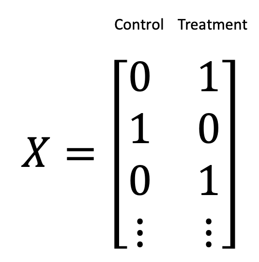
If you imagine that you have multiple samples, where the first and third samples correspond to your treatment group and your second sample corresponds to your control group, you could represent your treatment/control variables as dummy variables as follows

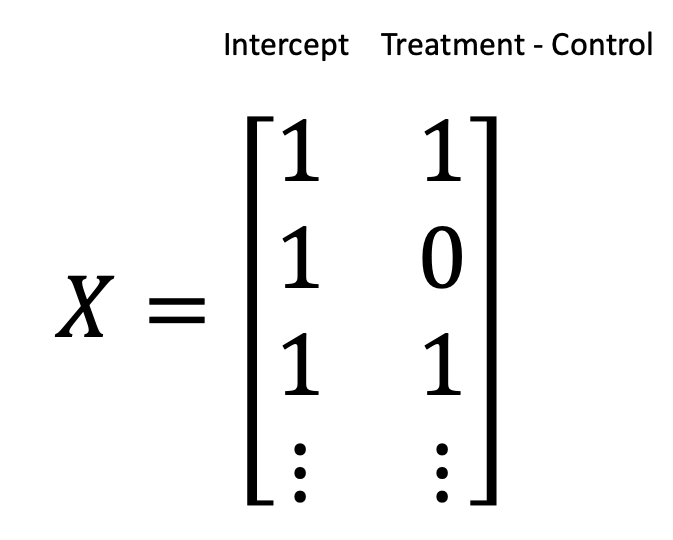
Another equally valid encoding is to use contrasts, where we explicitly model the difference between treatment and control as follows

And now this is where our mysterious intercept term comes in.

It may be more obvious if we focus on the simple univariate case. The simple linear regression would be given as follows

\(y_t = \begin{bmatrix} 1 & x_t \end{bmatrix} \times \begin{bmatrix} \beta_0 \\ \beta_1 \end{bmatrix}\) where \(\beta_0\) is our intercept and \(\beta_1\) is our regression coefficient. Traditionally, \(\beta_1\) is the slope, but because we are dealing with categorical variables, it can be interpreted as the difference between the mean control and the mean treatment values. The following drawing may help with the interpretation. 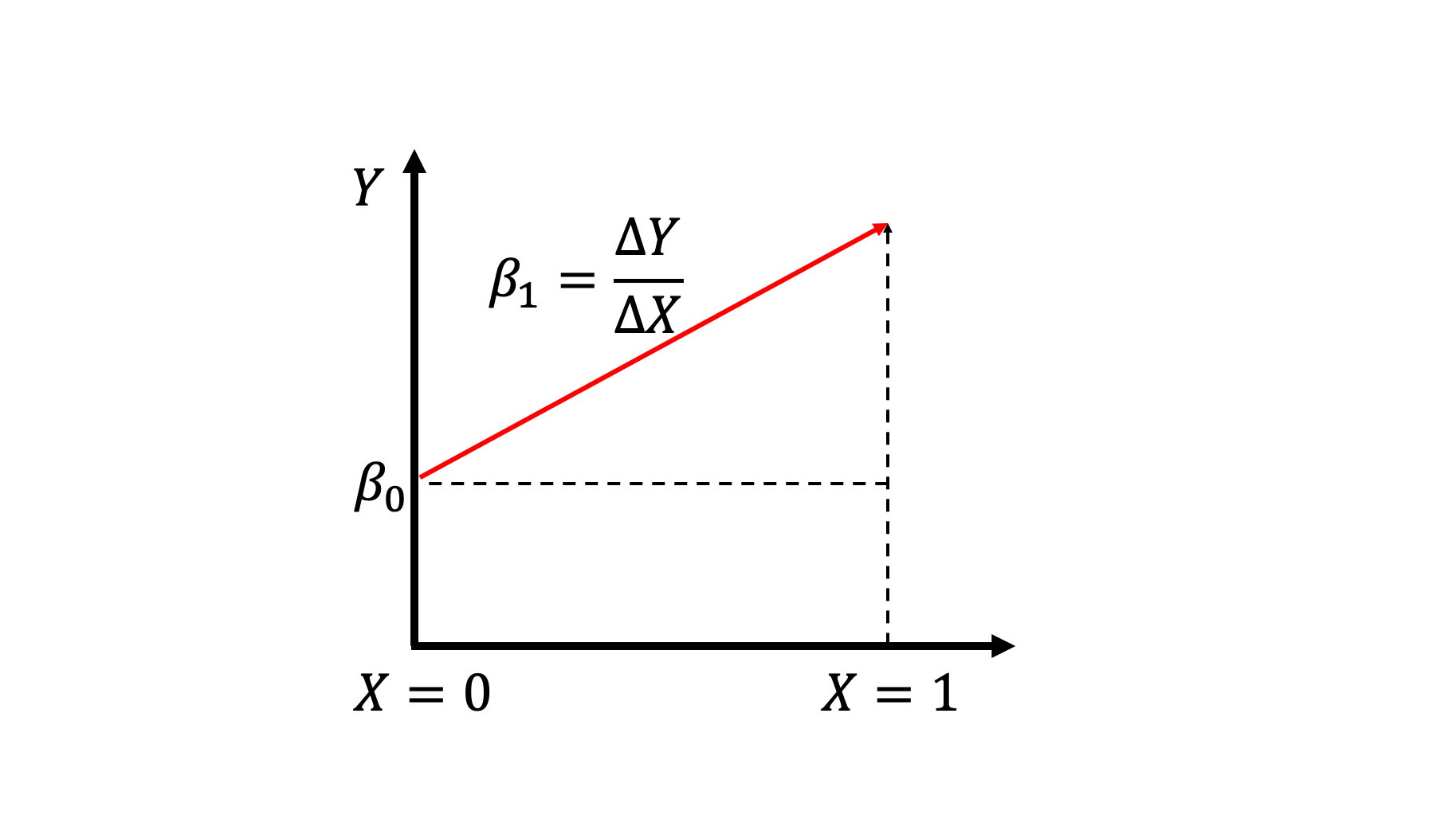Since \(\beta_1=\frac{\Delta y}{ \Delta x}\) and \(\Delta x=1\), that means that \(\beta_1\) only captures the difference between the \(y\) values. Another way to think of this is that since \(\beta_1\) estimates the difference between average treatment and control, then the intercept must estimate the average control. In other words, if we have estimated \(\beta_0, \beta_1\) the average treatment value can be given by \(\beta_0 + \beta_1\) since (control) + (treatment - control) = treatment. Then that just leaves us with the \(\beta_0\) estimating the average control value.

The take away here is that when only categorical variables are used as inputs, all of the coefficients estimate group averages and the differences between the group averages. This technique is essentially ANOVA - ANOVA is just linear regression with categorical variables.

Tying everything together, when applying this in a GLM context with Negative Binomial regression, all of these quantities are in log units. As acknowledged in previous works, the \(\beta_1\) coefficients correspond to some log-fold change quantity, with a bias as I mentioned in my paper. But one thing that I have not seen acknowledged elsewhere is that the intercept of this regression is the averaged log abundance of the control population. Specifically, if you exponentiate and normalize \(\beta_0\) to sum to 1, that quantity is expected to correspond to the average microbial population abundances in the control group.